As stated, the goal of this project was to capture the emotions experienced by participants as they listened to music, and to display these emotional journeys as artistic renders. To do this, the project used advanced deep learning techniques to classify valence and activation values in live electroencephalography (EEG) signals – namely, convolutional neural networks. These valence and activation values were then used to generate the images and videos displayed in the final presentation of the project. It is worth noting that, prior to this project, the investigator had no experience in computer programming or machine learning engineering. Therefore, any technical accomplishments made are solely as a result of the research and development of this project – and not any prior understanding or work.

1. Technical Setup

This section will detail the media, mediums, and technologies used and created in the project, why they were chosen, how they were utilised, and how they could be used in future projects. The headings will be presented in the order they appear in the signal path (Outlined bellow):

Figure 1: Project signal path

1.1 EEG Headset

The project used EEG technology to record brainwave data from participants, for the purpose of training and classification. As demonstrated in related literature, brainwave data contains the encoded values of emotional valence and activation (Altenmüller, 2002); it is the job of the investigator to implement a way to decode these values. In this case, the “Muse: Brain Sensing Headband” was used. The Muse headband is a consumer grade EEG device designed for meditation activities. However, it comes with a suite of developer tools for recording and playback purposes. This device was chosen for its low cost and high resolution – supplying 4 independent channels with the electrode positions: TP9, AF7, AF8, TP10 (Bird et al., 2018). The placement of these electrodes provides a spatial context of brainwave signals – as well as raw values.

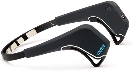
Figure 2: Muse headband

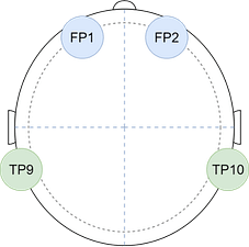
Figure 3: Electrode positions

1.2 Mind Monitor App

To interface with the headset, which would usually only be compatible with the Muse meditation app, the “Mind Monitor” app was used. The Mind Monitor app acts as a middle-man between the headset and the end-user, and can interpret the raw EEG data transmitted by the headset. The app also analyses the EEG data to create a profile for the current user, which is used to adaptively normalize the signals (Clutterbuck, 2021). A Fast Fourier Transform (FFT) is then applied, to convert the signals from the time domain to the frequency domain – showing how much activity lies within a frequency bandwidth, rather than the frequency and amplitude of the oscillations themselves (Clutterbuck, 2021). This information was then broadcasted to the host machine, over the Open Sound Control (OSC) protocol – in real-time.

Figure 4: Mind Monitor amplitude display

1.3 Neural Networks

As mentioned previously, this project used neural networks for data analysis. However, standard neural networks lack the ability to analyse temporal and spatial patterns in data, due to their instance-based linear nature. Therefore, a convolutional neural network (CNN) was used for the classification of valence and activation values. In short, CNNs are able to detect patterns in multidimensional data by grouping areas of close proximity; instead of viewing the data as one line, they examine it square by square. This makes them very effective for tasks that involve recognising features and patterns in a spatial context (Aggarwal, 2018). This was especially useful in the case of EEG analysis, as the network was able to interpret psychophysiological patterns, such as hemispherical activation and lateralization, natively. In this application, the JavaScript framework ml5.js was used to handle all neural network operations, as it incorporates TensorFlow.js (a widely used machine learning framework) and synergises well with the other major library used in the project; p5.js.

Figure 5: Model structure

1.3.1 Data Formatting

Before any data could be interpreted by the network, it first needed be formatted in a way that the network could understand. This was done in realtime as the data was being transmitted. The raw EEG data was received, over OSC, by the Neural Scores application – a program made in the development of this project. The Neural Scores application stored a 3 second short-term memory of the EEG data, which it then rendered as a spectrogram-like image. In the spectrogram image, the channels were ordered by frequency bandwidth and assigned a colour (i.e., delta was red, gamma was blue). This provoked the network to differentiate between the bandwidths. Inside each colour band are the electrode positions (TP9, FP1, FP2, TP10). The colour displayed in each individual pixel represented the amplitude of that frequency bandwidth, at that electrode, at that point in time.

Figure 6: EEG “spectrogram” image

Not only did this method provide a visual representation of the EEG data, but it also allowed the system to perform image classification – a technique whereby a convolutional neural network analyses an image by inspecting the red, green, blue, and alpha values of each pixel. This allowed the network to interpret physical aspects, such as hemispherical activation. Moreover, the sliding window nature of the spectrogram inherently contextualised the data in the time domain by presenting a running history of the values. This allowed the network to interoperate temporal aspects, such as spikes and fluctuations. The valence and activation classifications were run in realtime, with live EEG data. Then, the generated values were plotted against the circumplex model of affect. This produced a prediction for the strongest emotion felt by a participant – at that point in time.

1.3.2 Training

Before the network could be expected to make any classifications on experiment data, it first had to be taught how to understand the spectrograms and what to look for. Due to the black-box nature of machine learning, the network only required a dataset that contained labelled examples of the parameters of its task – it worked out the rules by itself. This meant the investigator simply needed broadcast training data to the Neural Scores application and give it a label for what it was receiving. This process would convert all the streamed training data into a single dataset, which could then be passed to the network for training. The training dataset could have been created with live EEG data, but this method was not chosen as there would have been no opportunity for quality control. For the purpose of this experiment, as there were two independent variables, two CNN models were created for the exclusive classification of each valence and activation. Once all training was complete for each participant, and the loss/accuracy functions were nominal, the trained models were saved and exported.

1.3.3 Classification

The classification process operated in a similar manner to the training setup, but, instead of storing the generated spectrogram images in a single dataset for training, they were instead instantly passed through the models for classification. Due to the low resolution of the spectrogram images and the nature of trained neural networks, this process was very lightweight and did not consume a lot of processing power. The system would output a classification for positive valence or negative valence, and positive activation or negative activation. The system also produces a confidence score for each classification. The confidence score is typically a ranking of how sure the network is of its classification. However, in this situation, as the only other possibility is the binary opposite of the classification, the confidence ranking was interoperated as a linear regression between each two classifications – a technique known as binary classification. The confidence scores for each classification (2 for valence, 2 for activation) were processed to produce one float value between -1.0 and 1.0 for each valence and activation. The values produced by the valence-activation classification system were then mapped directly to the circumplex model of affect proposed by Posner, Russel, and Peterson (2005). The values produced were also transported out of the Neural Scores application via OSC, to be used in any other creative application.

1.4 Neural Scores Application

As mentioned throughout, a standalone desktop application was created by the investigator, in the development of this project. This application, named “Neural Scores”, houses all the data processing, formatting, and neural network operations of the project. This was the product of many months of development, revisions, and debugging.

Initially, because the project was written in JavaScript, everything existed in a JavaScript browser window running on the localhost machine (JavaScript is typically a web only language). However, this setup was clunky, unstable, and required another program to form a bridge between the Mind Monitor app and the neural network facilities; because the project ran from a web browser, it was not able to see the OSC messages sent on the local area network (LAN) – thus requiring a secondary program to first transmit the LAN OSC data to the main program via WebSockets. However, this was resolved when the investigator rebuilt the project to run in an electron.js desktop application – which uses node.js to interoperate JavaScript code natively without the need for a web browser. This meant the Node-OSC library used in the initial bridge program could be directly integrated into the neural network and data formatting program, which could then be wrapped in a desktop application using the electron.js framework mentioned earlier. This process resulted in a user-friendly, scalable, and lightweight tool that could be deployed by anyone with the same EEG hardware – no need for finicky work-arounds!

The user interface of the application is very simple, the user is presented with three buttons on the left: classification view, spectrogram view, and settings. The classification view displays the current valence and activation values, along with the current predicted emotion as a pointer superimposed on an adapted circumplex model of affect. The spectrogram view displays the current frame of the EEG spectrogram render. The settings menu is where the user would control backend aspects of the program – such as, OSC port, saving and exporting, and model training. However, the settings page was not imperative to the progression of this project, so its development was discontinued until the project is complete. Currently, the models are trained in a separate browser-based app – which was also developed by the investigator.

The data exported by the application, over OSC, is as follows: valence, activation, circumplex valence (transform), circumplex activation (transform), circumplex colour (the colour the circumplex model pointer is currently over), and the original EEG data.

Figure 7: Classification View

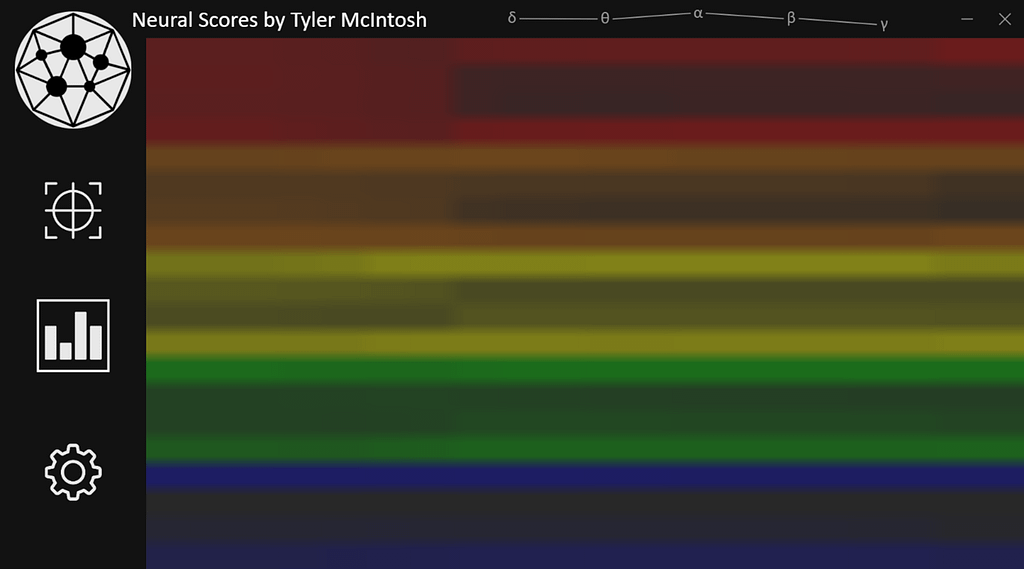
Figure 8: Spectrogram view

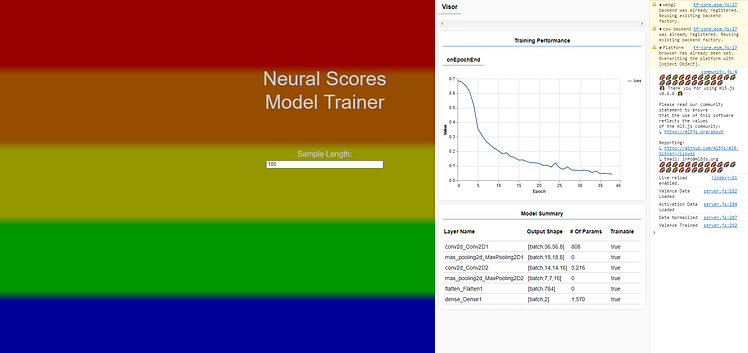
Figure 9: Separate model trainer used

1.5 Frontend Visual Output

The primary goal of this project was turn affective musical experience into artistic renders. Therefore, a significant amount of thought and research went into the design of the final output. Initially, the investigator planned to use JavaScript libraries, such as p5.js, to paint the emotions reported by the Neural Scores application to a digital canvas. However, it was later decided that the project would be better served by a more powerful program such as TouchDesigner – a hybrid programming environment centred around the Python programming language. This program offered much more advanced features for 2D and 3D visual rendering, and scaled better in terms of resolution and processing power requirements thanks to its low-level GPU utilisation. Therefore, all the images and videos displayed in the final presentation were made using this environment.

Figure 10: TouchDesigner renderer configuration

1.5.1 Emotion Backdrop

The first image generated by the system (see Figure 10) is the backdrop of the full images shown in the final presentation. These images show a marbling of colours that represent a short-term memory of the emotions felt by the participant (approx. 3-7 seconds). These emotions are displayed as colours, as dictated by the circumplex pointer colour in the Neural Scores application. In Figure 11, the majority of the image is blue with slight hints of red running through it. The heavy presence of blue would indicate that the current strongest emotion is that of low activation and low valence (blue/sadness). Whereas, the presence of red streaks would indicated that the participant arrived in this blue state from high activation and low valence (red/anger). Moreover, if the emotions of the participant are changing rapidly, there would be more colours blended into the image – the strongest emotion would be less clear, to reflect the uncertainty of the participant. There is also a bokeh particle system effect present in moments where there is a strong single emotion, which also reflects the participant’s activation through turbulence force magnitude.

Figure 11: Example backdrop

Figure 12: Backdrop component layering

1.5.2 Emotion Graph

As the main goal of the project was to display the complete journey of emotions, rather than only the ‘in-the-moment’ responses, a graphical representation of all the emotions felt over the duration of the music was implemented. This emotion graph takes the form of a circle, which progresses from left to right while the song is playing. As the circle line moves across the canvas, it draws spectrogram-inspired lines. The placement and intensity of these lines are controlled by the raw EEG data as it received from the headset. Additionally, the colour applied to the brush is controlled by the circumplex pointer colour reported from the Neural Scores application. This creates a detailed view of the complete history of both brainwave data and emotion data. Furthermore, the speed at which the circle progresses is controlled by the duration of the music being played – no matter the length, the circle will always progress around 360°. The emotion graphs are rendered over the backdrop, but are also exported separately over a transparent background. This would allow their incorporation into other work or material creation (such as, keyrings trinkets, t-shirts, and independent prints).

Figure 13: Emotion graph rendering (non matching EEG)

1.5.2 Audio Reactive Element

Finally, in-between the backdrop and the emotion graph, exists an audio reactive sphere. This element was added to give the videos extra relevancy to the music, and to separate the colours of the emotion graph from the colours of the backdrop. The construction of this was reasonably simple; it is a circle primitive, painted black and shifted down in opacity. The diameter of the circle is controlled by the audio – specifically, the amplitude of a certain frequency bandwidth that has been set using equalizers (e.g., bass only). To smooth the signal, an adaptive normalizing technique was used. This forces the signal to fade down from its peak, rather than declining directly with the raw audio signal.

Figure 14: Audio reactive circle example

2. Participant Procedure

As this project relied on people as a source of primary data, participants made up an important part of the planned procedure. While there were no character or lifestyle requirements regarding the selection of participants, there were health and safety constraints that must be noted. Namely, due to the national coronavirus lockdown restrictions, any participant interaction had to be limited to an opportunity sample of members of the investigator’s household who were of good physical and mental health. These were the only candidates that it would have been safe and legal to involve. Furthermore, EEG procedures carry a very small risk of causing seizures in people with epilepsy (NHS, 2018). Therefore, the selection process did not involve anyone with a history of seizures.

When a participant was selected, they were supplied with an information sheet and a consent form. They were also given an opportunity to ask any questions they might have had. Once this was complete, they were invited to a recording session. This session was split into two sections: training and experiment. In the training section, participants were asked to supply four songs that made them feel happy, sad, excited, and relaxed. They were also encouraged to recall memories and thoughts that might amplify these desired states. Next, the participant’s brainwave oscillations were recorded, while they were listening to each of the four songs provided. This data was used to train the emotion detection system specifically to them; each category of emotional response reflected an extreme of the valence/activation model. In the experiment section, the participant was asked to supply five songs that they would either like to see their emotion response to, or had a strong emotional sentiment for (e.g., favourite song, song played at major event, or song of other personal meaning). While they were listening to these songs, their brainwave data was being streamed to the Neural Scores application for classification. Then, the Neural Scores application sent the emotion information to the TouchDesigner project, which created the output image. This would all be done in realtime, as the song was being played, with very minimal delay. Whilst this process was running, a video capture of the TouchDesigner project would also be recorded.

Due to the constraints incurred by the pandemic, the project saw the involvement of only two participants – one of which being the investigator, and the other a household member. However, the investigator hopes to involve many more participants in the ongoing post-assessment work, under permitting conditions.

References

Aggarwal, C., 2018. Neural Networks and Deep Learning. Springer International Publishing.

Altenmüller, E., 2002. Hits to the left, flops to the right: different emotions during listening to music are reflected in cortical lateralisation patterns. Neuropsychologia, 40(13), pp.2242-2256.

Bird, J., Manso, L., Ribeiro, E., Ekart, A. and Faria, D., 2018. A Study on Mental State Classification using EEG-based Brain-Machine Interface. 2018 International Conference on Intelligent Systems (IS), pp.795-800.

Clutterbuck, J., 2021. Technical Manual. [online] Mind Monitor. Available at: <https://mind-monitor.com/Technical_Manual.php> [Accessed 3 March 2021].

NHS, 2018. Electroencephalogram. [online] Available at: <https://www.nhs.uk/conditions/electroencephalogram/> [Accessed 3 March 2021].